Visualizing lattices
Lattices can be visualized by serializing them into an HTML file. This can be done also via build.sequence_script
by supplying the argument markup='html'. The resulting HTML sequence file can be viewed in any modern browser and
elements can be inspected by using the browser’s inspector tool (e.g. <ctrl> + <shift> + C for Firefox).
Let’s visualize one of the example sequences:
>>> from importlib import resources
>>> from dipas.build import from_file, sequence_script
>>> import dipas.test.sequences
>>>
>>> with resources.path(dipas.test.sequences, 'cryring.seq') as path:
...     lattice = from_file(path)
...
>>> with open('cryring.html', 'w') as fh:
...     fh.write(sequence_script(lattice, markup='html'))
...
Note
The same result can also be obtained by using the madx-to-html command line utility that ships with the
dipas package. Just run madx-to-html cryring.seq to generate a corresponding cryring.html file.
Running madx-to-html --help shows all options for the utility.
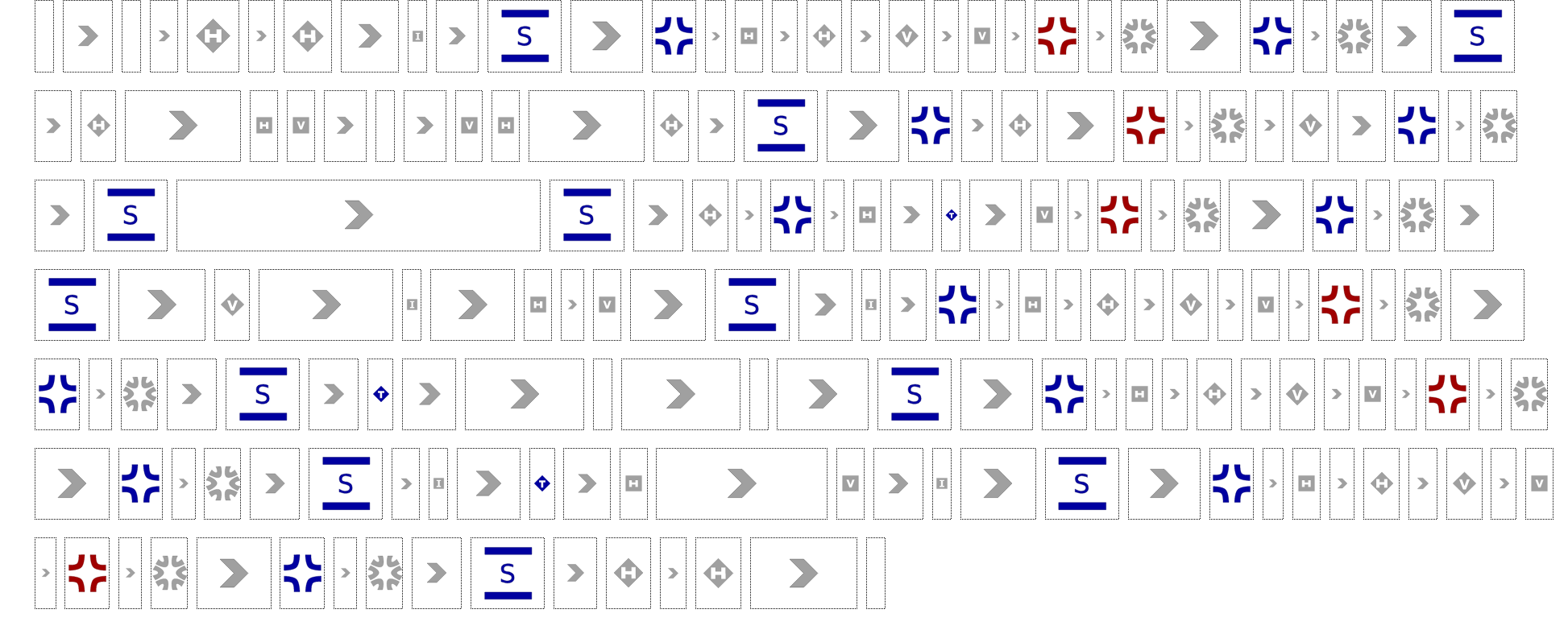
This produces the following HTML page, as viewed from the browser:
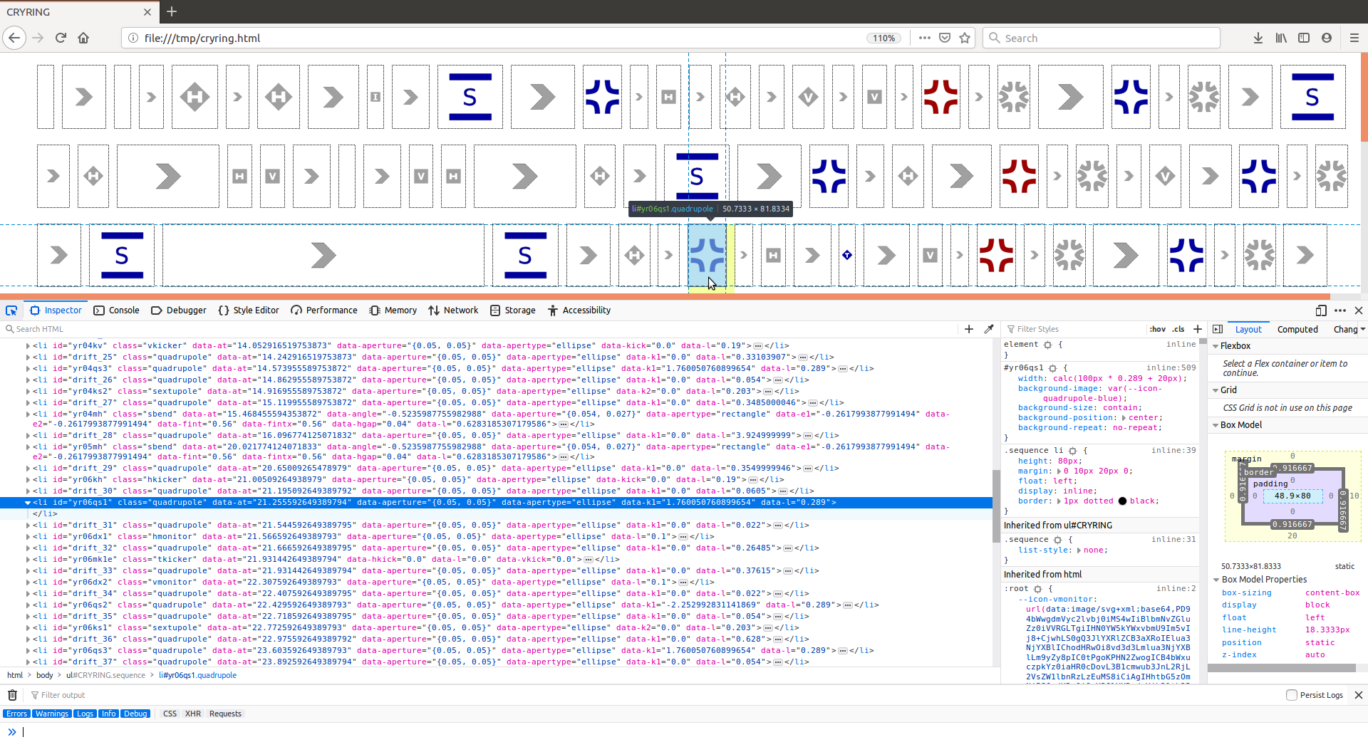
Using the browser’s inspector tool we can inspect the elements and view their attributes:
Legend: The following information is encoded in the visualization:
Drift spaces are displayed as
>,Kickers are displayed as diamonds; the letters “H”, “V”, “T” indicate the type of kicker (no letter indicates a bare KICKER).
RBend, SBend, Quadrupole and Sextupole are displayed by their number of coils; for RBend and SBend those are displayed as two horizontal bars, the letters “R”, “S” indicate the type of magnet.
Monitors and Instruments are displayed as rectangles,
HKicker, VKicker, Quadrupole, Sextupole, RBend and SBend elements are displayed in blue if their particular main multipole component (hkick, vkick, k1, k2, angle and angle) has a positive sign (except for RBend and SBend, where the sign is inverted, because a positive angle bends towards negative x-direction), are displayed in red if that component is negative (with the exception of RBend and SBend again) and are displayed in grey if that component is zero. A further exception are quadrupoles with
k1 == 0which are displayed as drift spaces (>).Kicker and TKicker elements are always displayed in blue,
Elements that do not actively influence the trajectory of the beam are displayed in grey (such as monitors, instruments),
Placeholders are displayed as drift spaces,
Markers are displayed as blank elements.
Plotting lattices and Twiss parameters
Lattices can be plotted together with Twiss parameters by using the plot.plot_twiss function. As an alternative,
the DiPAS distribution also provides a command-line interface for doing that:
dipas plot path/to/script.madx
The resulting plot is interactive, specifically hovering over lattice elements will show their label as well as plot a guiding line to indicate their s-position in the plot:
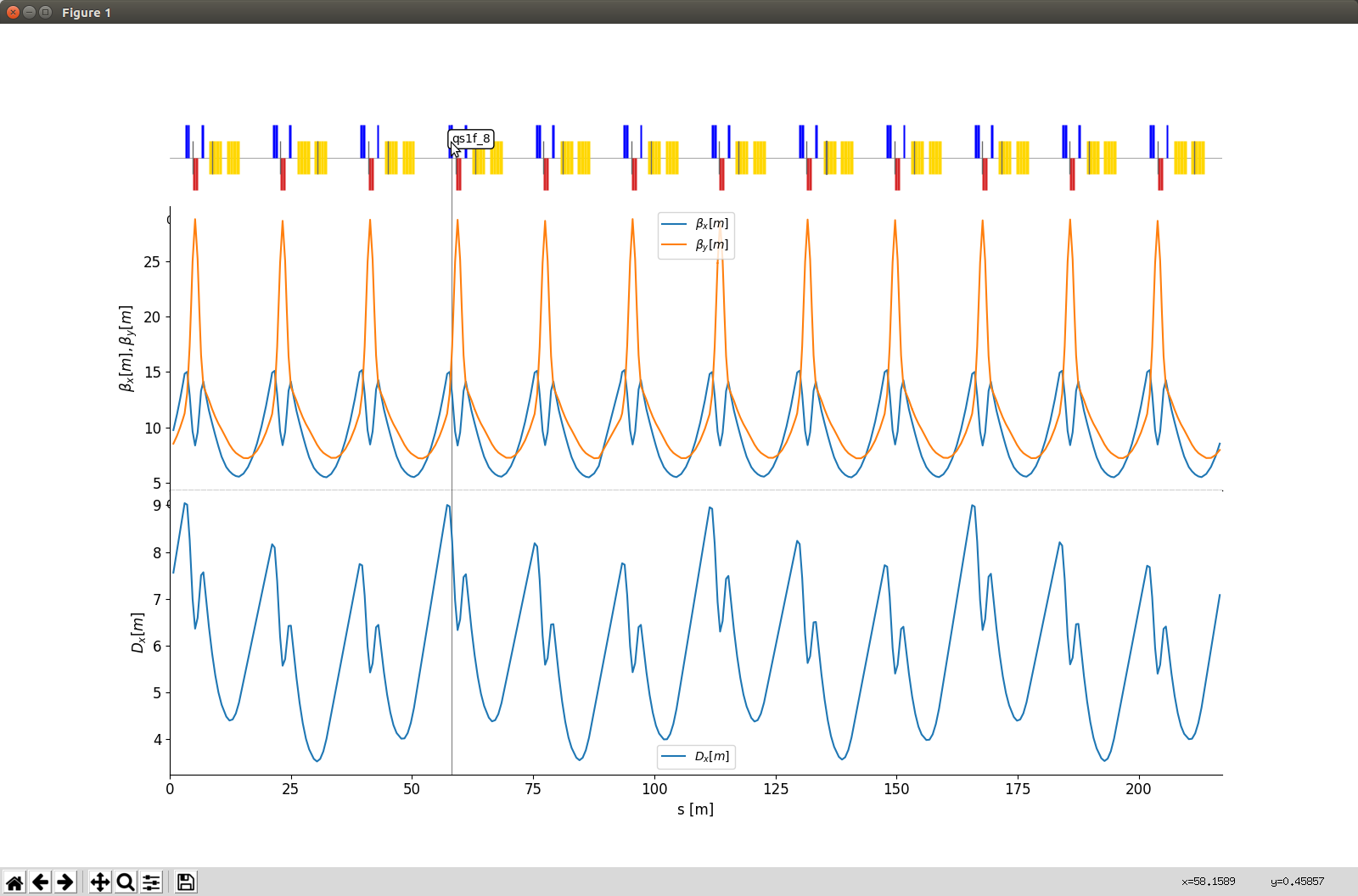
The plot is generated with matplotlib and depending on the plot-backend, e.g. PyQt5, it supports various other features
such as zooming or panning of axes.